Methods for defining the mesoscale structure of higher-order networks
This notebook compares multiple approaches to mesoscale structure in hypergraphs.
Hypergraph Spectral Clustering (hard partitions)
Hypergraph-MT and Hy-MMSBM (probabilistic models)
Hyperlink Communities (motif-driven communities)
Methods to visualize and interpret results
Definition
Community detection finds partitions or memberships with strong within-group interactions.
You will learn
Run community-detection workflows and compare outputs across methods.
Overview
Run community detection methods and compare outputs.
Visualize community assignments on example data.
Setup
[ ]:
import matplotlib as mpl

mpl.rcParams.update({
    "figure.figsize": (6, 4),
    "figure.dpi": 120,
    "savefig.dpi": 150,
})
[1]:
%load_ext autoreload
%autoreload 2
[2]:
# external
import sys
import random
import time

import numpy as np
import pandas as pd
import networkx as nx
import seaborn as sns
import matplotlib
import matplotlib.pyplot as plt

# core python modules
sys.path.append("..")
import hypergraphx
from hypergraphx.core.hypergraph import Hypergraph
from hypergraphx.readwrite.load import load_hypergraph
from hypergraphx.utils import normalize_array, calculate_permutation_matrix
from hypergraphx.communities.hy_sc.model import HySC
from hypergraphx.communities.hypergraph_mt.model import HypergraphMT
from hypergraphx.communities.hy_mmsbm.model import HyMMSBM
from hypergraphx.viz import draw_communities
Import the data
[3]:
dataset = 'workplace'
H = load_hypergraph(f"../test_data/{dataset}/{dataset}.json")
print(H)
Hypergraph with 92 nodes and 788 edges.
Distribution of hyperedge sizes: {2: 742, 3: 44, 4: 2}
[4]:
K = 5  # number of communities
seed = 20  # random seed
n_realizations = 10  # number of realizations with different random initialization
1) Train Hypergraph Spectral Clustering
[5]:
%%time

model = HySC(
    seed=seed,
    n_realizations=n_realizations
)
u_HySC = model.fit(
    H,
    K=K,
    weighted_L=False
)
CPU times: user 453 ms, sys: 136 ms, total: 589 ms
Wall time: 303 ms
2) Train Hypergraph-MT
Note
This model supports extra parameters to fix communities or the affinity matrix and to regularize inference. See the code cell below for the full list of supported keys.
[6]:
max_iter = 500  # maximum number of EM iteration steps before aborting
check_convergence_every = 1 # number of steps in between every convergence check
normalizeU = False  # if True, then the membership matrix u is normalized such that every row sums to 1
baseline_r0 = False  # if True, then for the first iteration u is initialized around the solution of the Hypergraph Spectral Clustering
verbose = False  # flag to print details
[7]:
%%time

model = HypergraphMT(
    n_realizations=n_realizations,
    max_iter=max_iter,
    check_convergence_every=check_convergence_every,
    verbose=verbose
)
u_HypergraphMT, w_HypergraphMT, _ = model.fit(H,
                                               K=K,
                                               seed=seed,
                                               normalizeU=normalizeU,
                                               baseline_r0=baseline_r0
                                              )
CPU times: user 17.7 s, sys: 224 ms, total: 17.9 s
Wall time: 19.1 s
Remark
Hypergraph-MT reduces the affinity matrix dimension via the assortative assumption, making inference feasible for larger systems.
[8]:
w_HypergraphMT.shape
[8]:
(3, 5)
[9]:
np.round(w_HypergraphMT, 3)
[9]:
array([[1.038, 0.532, 0.776, 0.847, 1.371],
       [0.017, 0.009, 0.004, 0.006, 0.015],
       [0.   , 0.   , 0.   , 0.   , 0.   ]])
3) Train Hy-MMSBM
Note
You can provide initial/fixed membership or affinity matrices. See the code cell below for configuration details.
[10]:
assortative = True # whether the affinity matrix w is expected to be diagonal
[11]:
%%time

np.random.seed(seed)
random.seed(seed)

# Train some models with different random initializations, choose the best one in terms of likelihood
best_model = None
best_loglik = float("-inf")
for j in range(n_realizations):
    model = HyMMSBM(
        K=K,
        assortative=assortative
    )
    model.fit(
        H,
        n_iter=max_iter
    )

    log_lik = model.log_likelihood(H)
    if log_lik > best_loglik:
        best_model = model
        best_loglik = log_lik

u_HyMMSBM = best_model.u
w_HyMMSBM = best_model.w
CPU times: user 6.09 s, sys: 68.8 ms, total: 6.15 s
Wall time: 6.37 s
Remark
Hy-MMSBM allows for a tractable and scalable inference by making use of a bilinear form. This allows to keep the dimension of the affinity matrix \(w\) equal to \(K \times K\) and to let \(w\) be free to capture different community structures, e.g., disassortative and assortative.
[12]:
w_HyMMSBM.shape
[12]:
(5, 5)
[13]:
np.round(w_HyMMSBM, 3)
# Note: the off-diagonal entries are zeros because we impose assortative=True
[13]:
array([[0.016, 0.   , 0.   , 0.   , 0.   ],
       [0.   , 0.013, 0.   , 0.   , 0.   ],
       [0.   , 0.   , 0.07 , 0.   , 0.   ],
       [0.   , 0.   , 0.   , 0.11 , 0.   ],
       [0.   , 0.   , 0.   , 0.   , 0.07 ]])
4)
[14]:
# TODO
Analyse communities
[15]:
departments = [H.get_node_metadata(n)['classID'] for n in sorted(H.get_nodes())]
u_ref = np.zeros(shape=(H.num_nodes(), K))
for i in range(H.num_nodes()):
    u_ref[i][departments[i]] = 1
[16]:
u_HypergraphMT = normalize_array(u_HypergraphMT, axis=1)
u_HyMMSBM = normalize_array(u_HyMMSBM, axis=1)
Let’s also permute the columns of the inferred membership matrices such that we have a higher correspondence with the reference.
[17]:
P = calculate_permutation_matrix(u_ref=u_ref, u_pred=u_HySC)
u_HySC = np.dot(u_HySC, P)

P = calculate_permutation_matrix(u_ref=u_ref, u_pred=u_HypergraphMT)
u_HypergraphMT = np.dot(u_HypergraphMT, P)

P = calculate_permutation_matrix(u_ref=u_ref, u_pred=u_HyMMSBM)
u_HyMMSBM = np.dot(u_HyMMSBM, P)
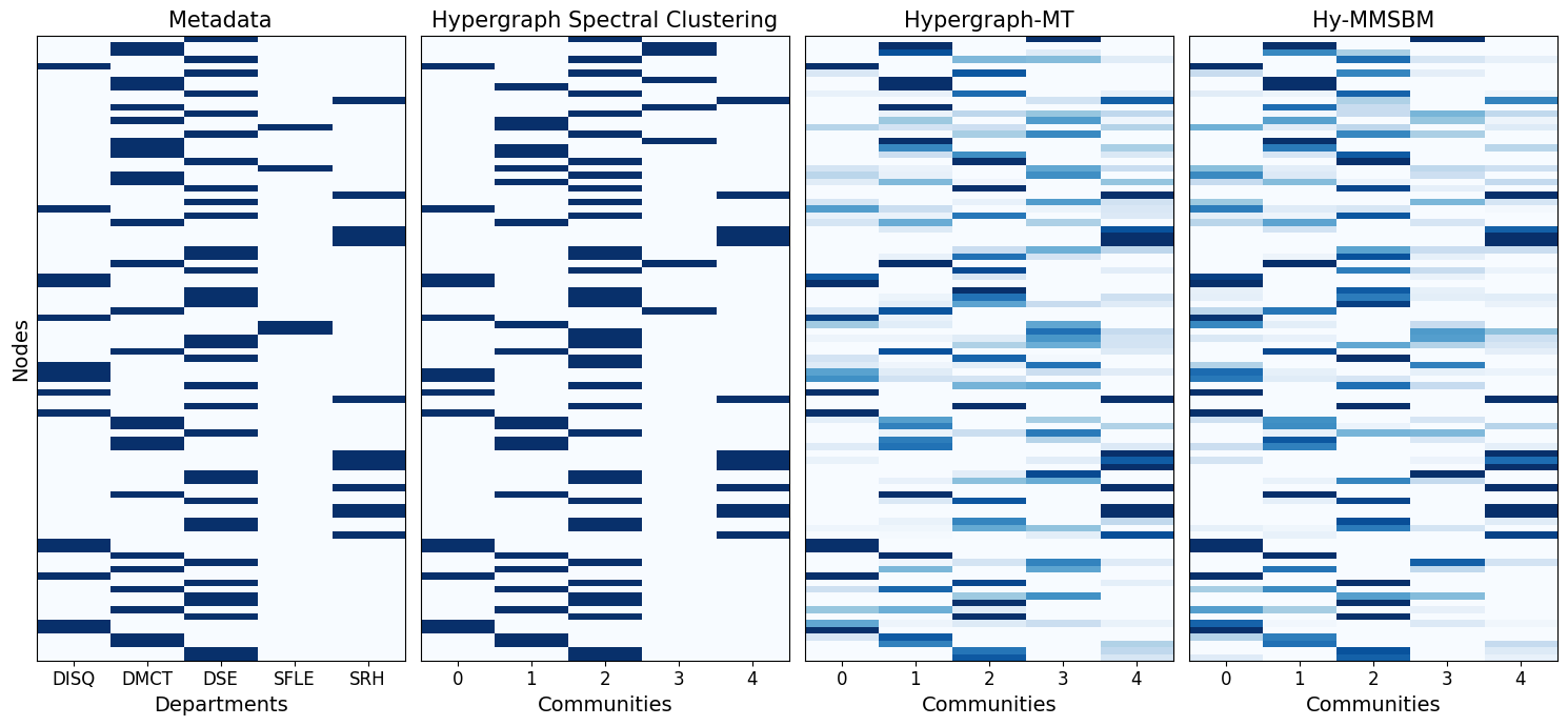
Let’s now visualize them.
Matshow
[18]:
params = {'legend.fontsize': '14',
         'axes.labelsize': '14',
         'axes.titlesize':'15',
         'xtick.labelsize':'12',
         'ytick.labelsize':'12'}
plt.rcParams.update(params)
[19]:
titles = ['Metadata', 'Hypergraph Spectral Clustering', 'Hypergraph-MT', 'Hy-MMSBM']

fig, ax = plt.subplots(1, 4, figsize=(15, 7), sharey=True)

ax[0].matshow(u_ref, aspect='auto', cmap='Blues')
ax[0].set(
    title='Metadata',
    xticks=[0,1,2,3,4],
    xticklabels = ['DISQ', 'DMCT', 'DSE', 'SFLE', 'SRH'],
    yticks = [],
    xlabel='Departments',
    ylabel='Nodes',
)

ax[1].matshow(u_HySC, aspect='auto', cmap='Blues')
ax[2].matshow(u_HypergraphMT, aspect='auto', cmap='Blues')
ax[3].matshow(u_HyMMSBM, aspect='auto', cmap='Blues')

for i in [1, 2, 3]:
    ax[i].set(
        title=titles[i],
        yticks = [],
        xlabel='Communities',
    )

for i in np.arange(4):
    ax[i].tick_params(top=False, labeltop=False, bottom=True, labelbottom=True)


plt.tight_layout()
plt.show()
Note
The mapping between row id and node label can be retrieved with _, mappingID2Name = H.binary_incidence_matrix(return_mapping=True).
Pie charts
[20]:
# Choose group colors
cmap = sns.color_palette("Paired", desat=0.7)
col = {k: matplotlib.colors.to_hex(cmap[k*2], keep_alpha=False) for k in np.arange(K)}
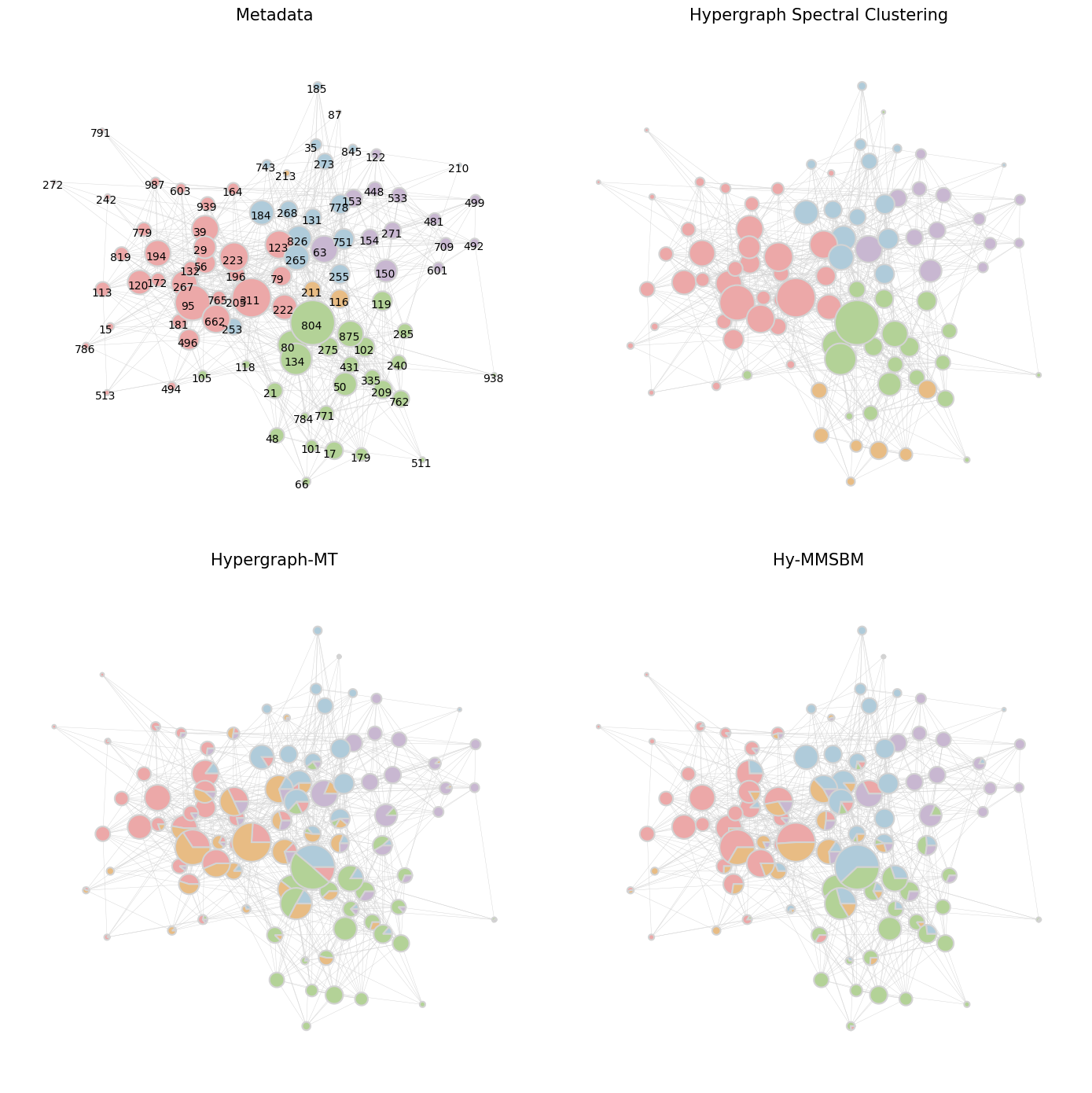
[21]:
plt.figure(figsize=(14,14))
plt.subplot(2,2,1)
ax=plt.gca()
draw_communities(hypergraph=H, u=u_ref, col=col, ax=ax, with_node_labels=True, title='Metadata')
plt.subplot(2,2,2)
ax=plt.gca()
draw_communities(hypergraph=H, u=u_HySC, col=col, ax=ax, with_node_labels=False, title='Hypergraph Spectral Clustering')
plt.subplot(2,2,3)
ax=plt.gca()
draw_communities(hypergraph=H, u=u_HypergraphMT, col=col, ax=ax, with_node_labels=False, title='Hypergraph-MT')
plt.subplot(2,2,4)
ax=plt.gca()
draw_communities(hypergraph=H, u=u_HyMMSBM, col=col, ax=ax, with_node_labels=False, title='Hy-MMSBM')