Analysis of the multiorder Laplacian matrix
Here we show how to analyze the multiorder Laplacian matrix defined for synchronization in higher-order networks.
Source:
Lucas M., Cencetti G., Battiston F., Multiorder Laplacian for synchronization in higher-order networks, Physical Review Research 2, 033410 (2020)
Definition
Multiorder Laplacians encode coupling at each interaction order for stability analysis.
You will learn
Analyze multiorder Laplacians and relate spectra to synchronization stability.
Overview
Analyze multiorder Laplacian spectra and synchronization properties.
Inspect how interaction order shapes stability.
Setup
[ ]:
import matplotlib as mpl

mpl.rcParams.update({
    "figure.figsize": (6, 4),
    "figure.dpi": 120,
    "savefig.dpi": 150,
})
[1]:
import sys

import numpy as np
import matplotlib.pyplot as plt

sys.path.append("..")
from hypergraphx.core.hypergraph import Hypergraph
from hypergraphx.linalg.linalg import compute_multiorder_laplacian, laplacian_matrices_all_orders
from hypergraphx.dynamics.synch import higher_order_MSF

from scipy.linalg import eigh

from itertools import combinations

np.random.seed(123)
[2]:
# definition of the higher-order network
edge_list = [[0,7],[1,2],[1,7],[2,7],[3,7],[4,7],[5,7],[6,7],[1,2,7],[4,5,6],[4,5,7],[4,6,7],[5,6,7],[4,5,6,7]]
hypergraph = Hypergraph(edge_list)

N = hypergraph.num_nodes()

# definition of the coupling coefficients, i.e., the strength of each order of interaction
sigmas = [1,1,1]
[3]:
# We can compute the Laplacian matrix for the different orders of interaction with
laplacians = laplacian_matrices_all_orders(hypergraph)

# for instance, the Laplacian matrix of order 2, i.e., the Laplacian matrix for three-body interactions, is given by
print(laplacians[2].todense())
[[ 0.  0.  0.  0.  0.  0.  0.  0.]
 [ 0.  2. -1.  0.  0.  0.  0. -1.]
 [ 0. -1.  2.  0.  0.  0.  0. -1.]
 [ 0.  0.  0.  0.  0.  0.  0.  0.]
 [ 0.  0.  0.  0.  6. -2. -2. -2.]
 [ 0.  0.  0.  0. -2.  6. -2. -2.]
 [ 0.  0.  0.  0. -2. -2.  6. -2.]
 [ 0. -1. -1.  0. -2. -2. -2.  8.]]
[4]:
# We can compute the multiorder Laplacian with
multiorder_laplacian = compute_multiorder_laplacian(hypergraph,sigmas)

print(multiorder_laplacian.toarray().round(3))
[[ 0.5    0.     0.     0.     0.     0.     0.    -0.5  ]
 [ 0.     2.067 -1.033  0.     0.     0.     0.    -1.033]
 [ 0.    -1.033  2.067  0.     0.     0.     0.    -1.033]
 [ 0.     0.     0.     0.5    0.     0.     0.    -0.5  ]
 [ 0.     0.     0.     0.     9.7   -3.067 -3.067 -3.567]
 [ 0.     0.     0.     0.    -3.067  9.7   -3.067 -3.567]
 [ 0.     0.     0.     0.    -3.067 -3.067  9.7   -3.567]
 [-0.5   -1.033 -1.033 -0.5   -3.567 -3.567 -3.567 13.767]]
[5]:
# The stability of a system of Kuramoto oscillators depends on the spectrum of the multiorder Laplacian
spectrum = eigh(multiorder_laplacian.toarray(), eigvals_only=True)

print(spectrum)
[-9.36750677e-16  5.00000000e-01  6.05839850e-01  1.44725527e+00
  3.10000000e+00  1.27666667e+01  1.27666667e+01  1.68135715e+01]
Master Stability Function
Here we show how to evaluate the Master Stability Function for synchronization in higher-order networks.
Source:
Gambuzza L.V., Di Patti F., Gallo L., Lepri S., Romance M., Criado R., Frasca M., Latora V., Boccaletti S., Stability of synchronization in simplicial complexes, Nature Communications 12(1), 1-13 (2021)
We study synchronization of coupled dynamical systems with higher-order interactions. The model follows a standard multiorder coupling form; the equations below define the dynamics used to compute the master stability function and related spectra.
[6]:
# To evaluate the MSF we need to define the coupling function F, its Jacobian matrix JF,
# as well as the Jacobian matrix of the coupling function, JH.
# In this tutorial, we will consider a system of Rossler oscillators, coupled through cubic functions
def rossler_system(t, X, a, b, c):
    x,y,z = X

    dxdt = - y - z
    dydt = x + a*y
    dzdt = b + z*(x - c)

    return np.array([dxdt,dydt,dzdt])

def jacobian_rossler(X, a, b, c):
    x,y,z = X

    dFxdX = [0, -1, -1]
    dFydX = [1, a, 0]
    dFzdX = [z, 0, x - c]

    return np.array([dFxdX, dFydX, dFzdX])

def jacobian_coupling(X):
    x,y,z = X

    dHxdX = [3*(x**2), 0, 0]
    dHydX = [0, 0, 0]
    dHzdX = [0, 0, 0]

    return np.array([dHxdX, dHydX, dHzdX])
[ ]:
# Setting of the isolated system
dim = 3
F = rossler_system
JF = jacobian_rossler
params = (0.2, 0.2, 9)

# Setting of the coupling
sigmas = [0.005, 0.0005, 0.00005]
JHs = [jacobian_coupling, jacobian_coupling, jacobian_coupling]

# Initial condition of the system
X0 = np.random.random(size=(3,))

# interval of values on which the MSF is evaluated
interval = np.logspace(-4,0.5,100)

MSF, hon_MSF, spectrum = higher_order_MSF(hypergraph, dim, F, JF, params, sigmas, JHs, X0, interval, integration_time=8000, integration_step=10**-3, verbose=False)
[ ]:
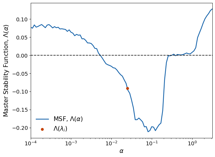
# We plot the results
fig, ax = plt.subplots(figsize=(8, 6))

# MSF
ax.plot(interval, MSF,
        lw=2, c=plt.cm.Blues(0.8), zorder=1,
        label="MSF, $\Lambda(\\alpha)$")

# Lyapunov exponents associated to the eigenvalues of the Laplacian matrix
ax.scatter(spectrum[1:], hon_MSF,
        color=plt.cm.Oranges(0.8), zorder=10,
        label="$\Lambda(\lambda_i)$")

ax.hlines(y=0, xmin=10**-4, xmax=10,
          colors=plt.cm.Greys(0.9), ls="--")

ax.semilogx()
ax.set_xlim(10**-4,10**0.5)
ax.tick_params(axis='both', which='major', labelsize=13)

ax.set_xlabel("$\\alpha$", fontsize=15)
ax.set_ylabel("Master Stability Function, $\Lambda(\\alpha)$", fontsize=15)
ax.legend(fontsize=15, frameon=False, loc=4)

plt.show()
[ ]:
# We now want to evaluate the MSF for the all-to-all case
def rossler_system(t, X, a, b, c):
    x,y,z = X

    dxdt = - y - z
    dydt = x + a*y
    dzdt = b + z*(x - c)

    return np.array([dxdt,dydt,dzdt])

def jacobian_rossler(X, a, b, c):
    x,y,z = X

    dFxdX = [0, -1, -1]
    dFydX = [1, a, 0]
    dFzdX = [z, 0, x - c]

    return np.array([dFxdX, dFydX, dFzdX])

def jacobian_coupling_order1(X):
    x,y,z = X

    dHxdX = [1, 0, 0]
    dHydX = [0, 0, 0]
    dHzdX = [0, 0, 0]

    return np.array([dHxdX, dHydX, dHzdX])

def jacobian_coupling_order2(X):
    x,y,z = X

    dHxdX = [3 * (x**2), 0, 0]
    dHydX = [0, 0, 0]
    dHzdX = [0, 0, 0]

    return np.array([dHxdX, dHydX, dHzdX])
[ ]:
# We build the all-to-all hypergraph with hyperedges of size two and three
N = 5
edge_list = list(combinations(range(N), 2)) + list(combinations(range(N), 3))
hypergraph = Hypergraph(edge_list)
[ ]:
# Setting of the isolated system
dim = 3
F = rossler_system
JF = jacobian_rossler
params = (0.2, 0.2, 9)

# Setting of the coupling
sigmas = [0.005, 0.0005]
JHs = [jacobian_coupling_order1, jacobian_coupling_order2]

# Initial condition of the system
X0 = np.random.random(size=(3,))

# interval of values on which the MSF is evaluated
interval = np.logspace(-4,0.5,100)

MSF, hon_MSF, spectrum = higher_order_MSF(hypergraph, dim, F, JF, params, sigmas, JHs, X0, interval, integration_time=6000, integration_step=10**-3, verbose=False)
[ ]:
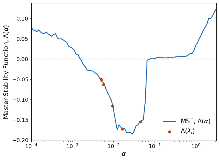
# We plot the results
fig, ax = plt.subplots(figsize=(8, 6))

# MSF
ax.plot(interval, MSF,
        lw=2, c=plt.cm.Blues(0.8), zorder=1,
        label="MSF, $\Lambda(\\alpha)$")

# Lyapunov exponents associated to the eigenvalues of the Laplacian matrix
ax.scatter(spectrum, hon_MSF,
        color=plt.cm.Oranges(0.8), zorder=10,
        label="$\Lambda(\lambda_i)$")

ax.hlines(y=0, xmin=10**-4, xmax=10,
          colors=plt.cm.Greys(0.9), ls="--")

ax.semilogx()
ax.set_xlim(10**-4,10**0.5)
ax.tick_params(axis='both', which='major', labelsize=13)

ax.set_xlabel("$\\alpha$", fontsize=15)
ax.set_ylabel("Master Stability Function, $\Lambda(\\alpha)$", fontsize=15)
ax.legend(fontsize=15, frameon=False, loc=3)

plt.show()